How to Apply the Beta Factor: A Practical Guide to Common Cause Failures in SIL Verification

When engineers perform SIL verification, most of the attention goes toward failure rates, proof test intervals, or diagnostics. But one input that carries enormous influence is beta factor (β) — the number that represents how much of your redundancy can be trusted to behave independently. Misunderstanding it can make even a perfect SIL calculation look better on paper than it really is in the field. This article walks through what β is, how it links to common cause failure (CCF), and how to apply it correctly with practical math and examples.

What Is It? (CCF vs. Beta Factor and Why It Matters)

Common cause failure (CCF) is a concept of multiple things failing for the same core reason. It is a concept in various industries and practices. In a Safety Instrumented System (SIS) it means multiple channels in redundant architectures fail together because of a shared cause. For example:

Sensors: Two pressure transmitters mounted side‑by‑side exposed to the same vibration or plugged impulse lines.
Logic solver: Both processor cards affected by the same unknown software bug.
Final element: Two solenoids sharing the same instrument air header that fail simultaneously.

The beta factor (β) is the fraction of all dangerous failures that occur from a CCF. It is the mathematical representation of the CCF concept. It converts the qualitative idea of “common cause” into a quantifiable term used in equations. Ignoring β will almost always make your average probability of failure on demand (PFDavg) appear lower than it really is — giving a false sense of security.

Where to Get Beta Factor Values

There are two primary sources:

SIL certificates or FMEDA reports from manufacturers. These often include β values based on test data and modeling assumptions.
IEC 61508‑6 Annex D – the formal method for determining β using dependent failure analysis. This process is complex and beyond the scope of this article, but it is the standard reference.

Other useful references include ISA TR84.00.02, OREDA, and CCPS reliability publications. Some companies maintain internal databases based on field performance.

A practical approach:

Start with the β from the SIL certificate.
Review Annex D factors to see if your installation justifies adjustment.
Document and justify the final value in your Safety Requirements Specification (SRS).

How Architecture Affects β

The β‑factor is not constant; it changes with architecture. This is a common point of confusion within Functional Safety. Think of redundancy as a team of security guards protecting a building:

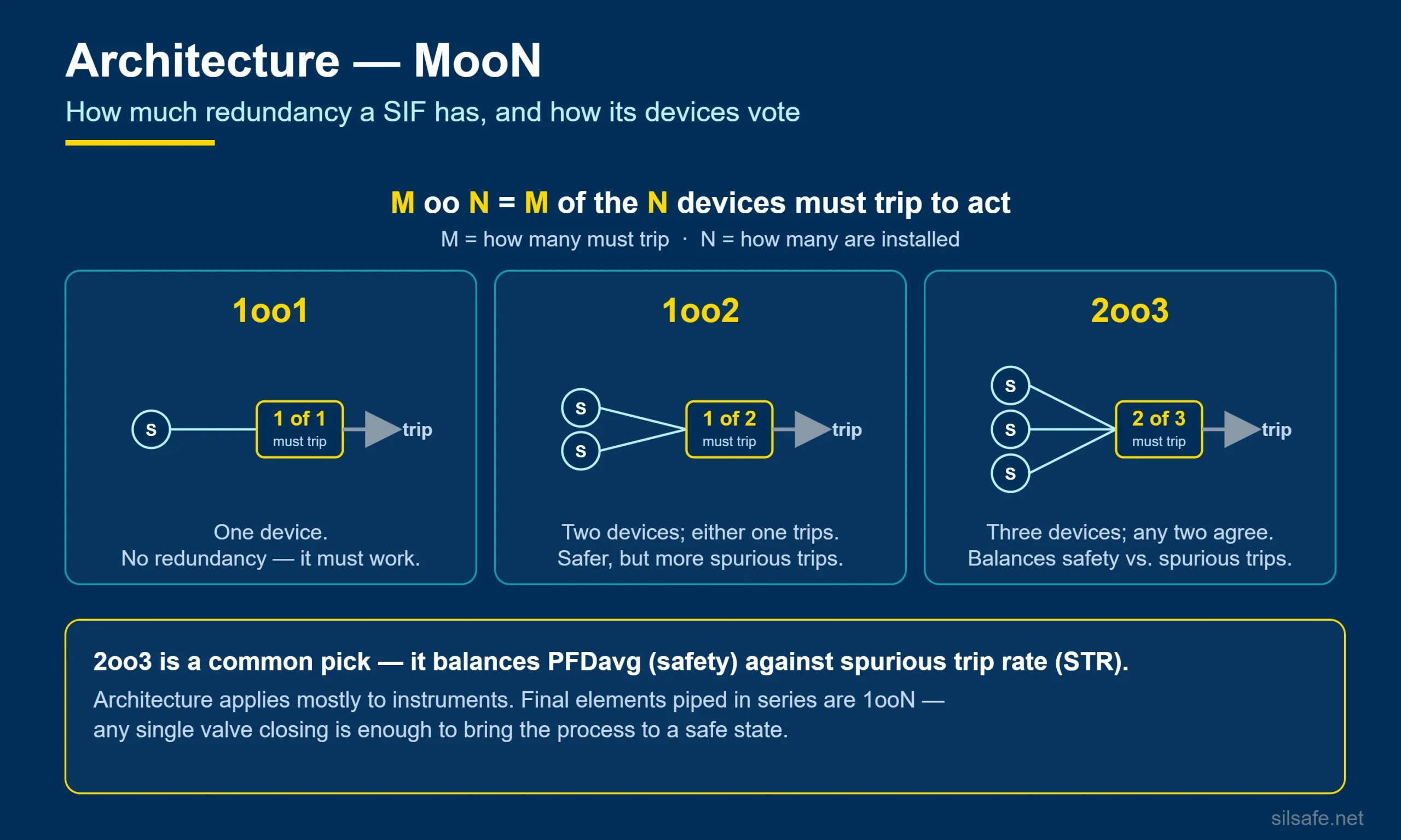
In a 1oo2 architecture, either guard can respond to stop a robbery. If both guards eat the same lunch and get food poisoning, that’s a CCF — a shared vulnerability.
In a 1oo4 architecture, four guards must all get sick for the robbery to succeed. The common cause event would have to be much stronger or more universal, or “more common,” to take them all down. Think of a really widespread case of food poisoning. Therefore, the effective β is lower.

This creates a feedback loop: changing architecture alters the PFDavg equation, but it also justifies a new β — which again changes the PFDavg. It is a bit odd, but it is correct. IEC 61508‑6 Annex D Table D.5 gives architectural correction factors (roughly 0.3 – 1.74) that help account for this effect. Most β values published in SIL certificates are assumed for 1oo2 configurations.

NooN Architectures and Why β is Not Present

For NooN architectures (e.g., 2oo2 or 3oo3), β is normally not present in the mathematics. Any single channel failure will cause the function to fail because all channels must work. The total λDU (dangerous undetected failure rate) already includes both independent and common‑cause contributions. Applying a separate β term would double‑count the effect.

Returning to the guard analogy: if three guards must all respond correctly and any one failure causes system failure, it doesn’t matter if their failures were independent or shared — the result is the same. For this reason, modeling tools and standards do not include β for NooN designs.

Note that this can be thought of as “β is set to 0 for NooN” but that is not how we at SIL Safe think of this. Yes, you can use the MooN PFDavg equations, set β = 0, and get the same results. But as we discussed above, β is accounted for in λDU.

Typical Values and Influencing Factors

Subsystem	Typical β Range
Sensors	0.02 – 0.10
Logic Solvers	0.01 – 0.05
Final Elements	0.05 – 0.15

Factors that increase β:

Common environment (same enclosure, same power, same impulse lines)
Identical design and firmware
Shared maintenance procedures or simultaneous testing

Factors that decrease β:

Physical separation and shielding
Vendor or technology diversity
Independent power and utilities
Separate calibration schedules
Staggered proof testing

PFDavg Equation Discussion

In a 1oo2 system, the total PFDavg is made up of independent and common‑cause terms. Using a simplified version of the equation:

Equation showing how the beta factor (β) influences PFDavg in a 1oo2 safety architecture by combining independent and common cause failure probabilities.

Where:

λ_DU = dangerous undetected failure rate (per hour)
TI = proof test interval (hours)
β = fraction of failures due to common causes

The first term (squared) represents two independent latent failures. The second (linear) term represents the probability that both channels fail from a shared cause. Because the independent term is squared, it becomes much smaller — making β a powerful driver in redundant designs.

PFDavg Calculation Examples (1oo2)

Case A – Good β Factor (Target: SIL 2)

Given: β = 0.03, λ_DU = 2E-6/hr, TI = 8,760 hr (1 year)

Independent term:
(1/3) × [(1 − 0.03) × 2E-6 × 8,760]² = 9.63E-5
Common‑cause term:
(1/2) × 0.03 × 2E-6 × 8,760 = 2.63E-4
Total PFDavg = 3.59E-4
RRF = 1 / PFDavg = 2,785 → SIL 2

STR (spurious trip rate): assume λ_SP = 1E-5/hr per channel. For 1oo2 (trip on any channel):
STR ≈ 2 × λ_SP = 2E-5/hr → 0.175 trips per year ≈ 1 trip every 5.7 years.

Case B – Poor β Factor (Target: SIL 1)

Given: β = 0.15, λDU = 2E-6/hr, TI = 8,760 hr (same assumptions)

Independent term:
(1/3) × [(1 − 0.15) × 2E-6 × 8,760]² = 7.4E-5
Common‑cause term:
(1/2) × 0.15 × 2E-6 × 8,760 = 1.31E-3
Total PFDavg = 1.38E-3
RRF = 1 / PFDavg = 725 → SIL 1

STR (same λ_SP): 2E-5/hr → 0.175 trips/year or a trip, or 5.7 years, (same  as Case A).

Comparison: Raising β from 0.03 to 0.15 increased total PFDavg by ≈ 4×, dropping the SIL from 2 to 1.

Impact of Common Cause Portions of PFDavg

Because the independent term is squared, it diminishes as reliability increases, while the common‑cause term remains linear. The result: CCF often dominates total PFDavg in redundant architectures.

Case A (β = 0.03): PFDavg_ind = 9.63E-5, PFDavg_cc = 2.63E-4 → CCF ≈ 73% of total.
Case B (β = 0.15): PFDavg_ind = 7.4E-5, PFDavg_cc = 1.31E-3 → CCF ≈ 95% of total.

Even at modest β values, most of the total unavailability stems from common causes — which is why reducing β through independence and diversity is far more effective than upgrading the architecture. The same pattern holds true for higher architectures like 2oo3.

Common Mistakes

Applying the same β to every subsystem without justification.
Assuming diagnostics lower β (they don’t; they reduce λ_DU).
Forgetting to justify β selection in the SRS.
Focusing only on adding redundancy instead of lowering β.

Summary

The β‑factor is what connects real‑world dependencies to your math. A small change in β can shift a design from SIL 2 to SIL 1 — even when every other parameter is identical. Real independence, not just redundancy, drives reliability.

Document your β assumptions, revisit them through the SIS life‑cycle, and when in doubt, verify them against IEC 61508‑6 Annex D or manufacturer data.

If you’d like a second set of eyes on your β assumptions or SIL verification model, contact SIL Safe for a practical review or training session.

Q&A

1. Does β apply only to 1oo2 architectures?
No. The concept applies to any redundant system where channels can fail together, though it’s most visible in 1oo2.

2. Can β ever be zero?
Not realistically. There’s always some shared factor — environment, maintenance, or design — that introduces correlation. For NooN scenarios, β does not appear in the mathematics, so some say β is zero, but it is still included in the λ_DU term.

3. What does β actually represent?
It’s the percentage of dangerous failures that are shared between channels rather than truly independent.

4. How often should β be revisited?
Any time design, environment, or procedures change — typically during periodic review or FSA Stage 4. It is common for β to change over the safety lifecycle.

5. Can one simply apply the β in the SIL certificate?
Use it as a starting point. Then compare against Annex D’s checklist and justify any adjustment.

6. What portion can common cause contribute to total PFDavg?
Often the majority. For 1oo2 with β ≈ 0.1–0.2, common cause failures can make up 70–95 % of total PFDavg — the same trend appears in higher architectures.

7. I’ve heard that for NooN architectures, β is set to 0, but I thought that is not possible?
β is involved in NooN, but it is already included in the λ_DU term. Meaning we don’t want to double count. The NooN equations will not have any β terms. Thus, it can be thought of as they were set to zero, but that is not technically correct.